🕹️ User’s Guide
This section aims to showcase wakiscapabilities together with useful recipes to use in the simulation scripts.
Since wakis has been developed for computing beam-coupling impedance for particle accelerator components, the example that will serve as a conductive thread for the explanation is a pillbox cavity with a passing proton beam.
The guide will go into detailed step-by-step on how to write the simulation script and visualize or access the computed data.
Contents
🪜 Simulation step-by-step
Import modules
The first part of a python script always includes importing external sources of code e.g., packages or modules. In wakis, we use:
numpy: Used for numerical operations, especially for matrix operations.scipy.constants: to import physical constants easily like vacuum permittivityeps_0or the speed of lightcmatplotlib: Used for 1d and 2d plotting and visualization.h5py: To store data in the memory-efficient format HDF5tqdm: This package is used for displaying progress bars in loops.pyvista: For handling and visualizing 3D CAD geometries and vtk-based 3D plotting.
Optionally, one can use os or sys packages to handle the PATH and directory creations. The first part of any simulaiton script could look similar to:
import numpy as np               # for handling arrays
import matplotlib.pyplot as plt  # for plotting
import os, sys                   # for path handling
import pyvista as pv             # for geometry modelling and 3D visualization
import h5py                      # for data save/import
from tqdm import tqdm            # for time loop prpgress bar
from scipy.constants import c as c_light    # speed of light constant
Next step is to import the wakis classes that will allow to run the electromagnetic simulations:
from wakis import GridFIT3D       # Grid generation
from wakis import SolverFIT3D     # EM field simulation
from wakis import WakeSolver      # Wake and Impedance calculation
Simulation domain, geometry and materials setup
wakis is a numerical electromagnetic solver that uses the Finite Integration Technique. The grid used is a structured grid composed by rectangular cells. The simulation domain is a rectangular box that will be broken into cells where the electromagnetic fields will be computed. Notice that all the input parameters for Wakis must be in SI Base Units.
Number of mesh cells
In every wakis simulation example, the script starts specifying the number of mesh cells per direction the user wants to use:
# ---------- Domain setup ---------
# Number of mesh cells
Nx = 50
Ny = 50
Nz = 100
Note
Note that the number of cells will heavily affect the simulation time (in particular, the timestep due to CFL condition), and also the memory requirements.
STL geometry importing
In beam-coupling impedance simulations one is usually interested in the geometric impedance, together with the impedance coming from material properties. In wakis, the geometry to simulate (sometimes referred as Embedded boundaries) can be imported from a .stl file containing a CAD model, and the units should be meters [m].
# stl geometry files (add path to them if necessary)
stl_cavity = 'cavity.stl'
stl_shell = 'shell.stl'
stl_solids = {'cavity': stl_cavity, 'shell': stl_shell}

# Optional: plot the geometry imported using PyVista
geometry = pv.read(stl_shell) + pv.read(stl_cavity)
geometry.plot() # add pyvista **kwargs to make a fancier plot
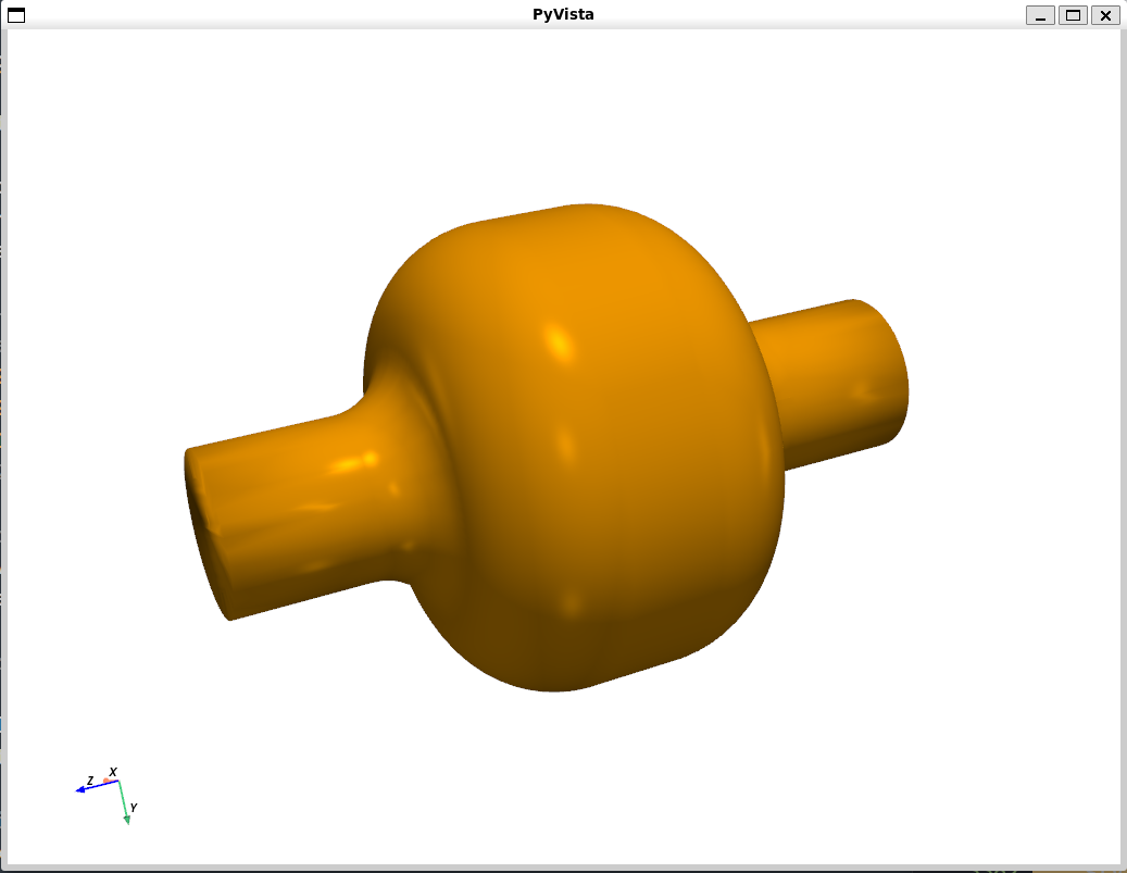
Some example .stl files are available in the GitHub repository for the notebooks/ and examples folders. However, PyVista allows to generate importable geometry really easy through Constructive Solid Geometry (CSG). CSG is a modeling technique where complex geometries are built by combining simple primitives (like cubes, spheres, cylinders, cones) using Boolean operations: Union (+) combines two solids, Intersection (*) keeps only the overlapping volume or Difference (−): subtracts one solid from another. An example on how to generate a pillbox cavity using CSG is shown bellow:
import pyvista as pv

# create 2 cylinders oriented in the z-direction
pipe = pv.Cylinder(direction=(0,0,1.), radius=0.12, height=1)
cavity = pv.Cylinder(direction=(0,0,1.), radius=0.5, height=0.3)

# combine them and plot
surf = pipe + cavity
surf.plot()

# save
surf.save('geometry.stl', binary=False)
See also
Check PyVista’s documentation for more advanced 3d plotting
Imported .stl files can also be translated, rotated and scaled in x, y, z by providing a list. E.g., stl_scale['cavity'] = [1., 2, 1.] will duplicate the y dimension of the imported cavity.stl.
stl_scale = {'cavity': [1., 1., 2.], 'shell': [1., 1., 2.]} # scale factor
stl_rotate = {'cavity': [1., 1., 90.], 'shell': [1., 1., 90.]}  # rotate angle (degrees)
stl_translate = {'cavity': [1., 0, 0], 'shell': [1., 0, 0]} # displacement in [m]
Associating a material to each solid
Each stl solid can be associated with a material by indicating [eps, mu, conductivity]. In materials.py, the most used materials are available in the material library. The user can specify a value for the relative permittivity \(\varepsilon\), the relative permeability \(\mu\) and the value for the conductivity \(\sigma\) in [S/m] or use the material name from the library:
# Indicate relative permittivity, relative permeability and conductivity [S/m]
# [eps_r, mu_r, conductivity]
# or the material name from the library:
stl_materials = {'cavity': 'vacuum',       # equivalent to [1.0, 1.0, 0]
                'shell': [1e3, 1.0, 1e3]}  # equivalent to a 'lossy metal'
Defining the grid object
After this, the user needs to indicate the domain bounds to simulate, in [m]. They can be calculated from the imported geometry or just hardcoded with float values:
# Domain bounds
geometry = pv.read(stl_shell) + pv.read(stl_cavity)
xmin, xmax, ymin, ymax, zmin, zmax = geometry.bounds
Finally, we can build our simulation grid using GridFIT3D class including all the information above:
# initialize grid object
grid = GridFIT3D(xmin, xmax, ymin, ymax, zmin, zmax,
                Nx, Ny, Nz,
                stl_solids=stl_solids,
                stl_materials=stl_materials,
                stl_translate=stl_translate,
                stl_scale=stl_scale,
                stl_rotate=stl_rotate,
                )
Optionally, the grid of the simulation can be inspected interactively in 3D (thanks to PyVista):
grid.inspect(add_stl=['cavity', 'shell'] #default is all stl solids
             stl_opacity=0.5             #default is 0.5
             stl_colors=['blue', 'red']) #default is `white`
wakis API is fully exposed, so all the grid class parameters relevant for the simulation can be accessed as class attributes and modified once the class has been instantiated. E.g., grid.dx gives the mesh step size in x direction, grid.N gives the total number of cells. Attributes can be checked by typing grid. and then pressing TAB when running on ipython.
Tip
Thanks to a fully exposed python API, all (relevant) class attributes can be checked by typing the class instance (e.g., grid or solver) followed a dot . and the name of the attribute.
When running on ipython all attributes and functions() can be viewed by typing the name of the class instance + . and then pressing TAB. Similarly, when writing code on a IDE (e.g., Visual Studio), a list with all the attributes and functions will be shown when typing e.g., solver..
Setting up the electromagnetic solver
Once the simulation domain has been defined through the geometry and the grid, the electromagnetic (EM) solver can be created. The solver implemented in wakis uses the Finite Integration Technique (FIT) [^1]. The recipe on how to instantiate the SolverFIT3D class is given below:
solver = SolverFIT3D(grid=grid,     # pass grid object
                     dt=dt,         # (OPTIONAL) define timestep
                     cfl=0.5,       # Default if no dt is defined
                     bc_low=bc_low,
                     bc_high=bc_high,
                     use_stl=True,     # Enables or disables geometry import
                     bg='vacuum',      # Background material
                     )
Simulation timestep
The simulation timestep is calculated following the CFL condition, that mainly depends on the cell size. A default value of 0.5 ensures simulation stability:
# Extract of SolverFIT3D __init__
self.dt = cfln / (c_light * np.sqrt(1 / self.grid.dx ** 2 + 1 / self.grid.dy ** 2 +
                                            1 / self.grid.dz ** 2))
Boundary conditions
The required parameters bc_low and bc_high allow to choose the 6 boundary conditions for our simulation box. For the lower-end boundaries bc_low = [x-, y-, z-] and for the high-end boundaries bc_high = [x+, y+, z+] is used. The supported values to give for -/+ boundaries are:
pecstands for Perfect Electric Conductor: it is a Dirichlet boundary conditions that forces the tangent electric \(E\) field at the boundary to be 0.pmcstands for Perfect Magnetic Conductor: similarly to pec, it is a Dirichlet boundary conditions that forces the tangent magnetic \(H\) field at the boundary to be 0.periodic: The field values of the high-end boundary are passed to the lower-end boundary, simulating a periodic structure where the fields re-enter the simulation domain.abcFirst order extrapolation (FOEXTRAP) absorbing boundary condition (ABC)[^2]: a type of Dirichlet absorbing boundary condition that allows to absorb longitudinally propagating fields when they reach the boundary. Only works under specific circumstances.pmlPerfect Matching Layer: A more advanced type of ABC, capable of absorbing electromagnetic waves propagating in a wider range of propagation angles [^3]. This boundary conditions are needed e.g., for simulating accelerator beampipe transitions and RF cavities above beampipe cutoff. Currently under development
An example of the boundary conditions that are typically used for the pillbox cavity example are:
# boundary conditions
bc_low=['pec', 'pec', 'pml']  #or z=`pec` if below cutoff
bc_high=['pec', 'pec', 'pml'] #or z=`pec` if below cutoff
Accessing solver’s fields, matrices and simulation parameters
Similarly to the grid object from GridFIT3D, wakis’s SolverFIT3D class is fully exposed. This means that once the solver object is instantiated, all the parameters of the EM solver can be accessed as class attributes solver.attr and modified. E.g., one can modify the simulation timestep after the instantiation by doing:
solver.dt = 1e-9 #[s]
Electromagnetic fields E, J, H
Once the solver has been instantiated, the electromagnetic fields electric \(E\), magnetic \(H\) and current \(J\) can be accessed and modified to e.g., add initial conditions to the simulation. The fields are 3D vectorial matrices of sizes [Nx, Ny, Nz]x3. The times 3 comes from their vectorial nature, since there are values for each simulation cell in \(x\), \(y\), and \(z\) direction. Below an example on how to access the electric field component \(E_z\) to add an initial condition to the field:
# modify the lower left bottom corner (cell [0,0,0]) of the simulation domain.
solver.E[0,0,0,'z'] = c_light

# modify the x component of H for a XY plane at a particular z
iz = Nz//3
solver.H[:, :, iz, 'x'] = np.ones((Nx, Ny))

# modify the y component of the J on the z axis at a particular x, y
ix, iy = Nx//2, Ny//2
solver.J[ix, iy, :,'y']

# get the absolute value of the electric field
E_abs = solver.E.get_abs() #size [Nx, Ny, Nz]
The routines inspect() for 2D and inspect3d() allow for quick visualization of the field values:
solver.E.inspect(plane='YZ',            # 2d plane, cut at the domain center
                 cmap='bwr',            # colormap
                 dpi=100,               # plot DPI value (pixel resolution)
                 # also, the plane can be specified as a 2D slice in x,y,z
                 # e.g., for the YZ plane at x = Nx//2
                 x=Nx//2,
                 y=slice(0,Ny),
                 z=slice(0,Nz)
                )
Material tensors ieps, imu, sigma
The same applies for the material tensors for permittivity \(\varepsilon\), permeability \(\mu\), and conductivity \(\sigma\). For computational cost reasons, the values saved in memory correspond to \(\varepsilon^{-1}\) and \(\mu^{-1}\). To access a specific value or a slice of values (and modify them if desired):
# permittivity(^-1) tensor in x direction
solver.ieps[:, :, :, 'x']

# permeability(^-1) tensor in y direction
solver.imu[:, :, :, 'y']

# Modify first 10 cells in x of the conductivity tensor:
for d in ['x', 'y', 'z']:
    solver.sigma[:10, :, :, d] = np.ones(10)*1e3 #S/m
Since wakis supports anisotropy, the tensors are 3D matrices of sizes [Nx, Ny, Nz]x3 since there are values for each simulation cell in \(x\), \(y\), and \(z\) direction. Similarly, one can inspect the values given to the tensors by using e.g., solver.sigma.inspect()
Tip
Material tensors \(\varepsilon\), \(\mu\), and \(\sigma\), and electromagnetic fields \(E\), \(H\) and \(J\) are created as Field objects, the class in field.py. This class allows for optimized access to matrix values, conversion to array format using the lexico-grapihc index and inspection methods ìnspect()` via 2D plots to confirm that the tensor are built correctly before running the simulation.
Running a simulation
Once the domain and geometry are defined in grid and the fields and internal operators have been instantiated with solver, an electromagnetic time-domain simulation can be run provided some initial conditions. The simplest way to run the code, step-by-step, is by calling the routine solver.one_setp():
# Run one step (advance from t=0 to t=dt)
solver.one_step()

# Run a number of timesteps while modifying the fields
hf = h5py.File('results/Ex.h5', 'w')
Nt = 100
for n in tqdm(range(Nt)):

    # [OPTIONAL] Modify field
    #source_fun(t) can be any function, see next section
    solver.E[:, :, :, 'x'] = source_fun(n*dt)

    # Advance
    solver.one_step()

    # [OPTIONAL] Plot 2D on-the-fly. -->See dedicated section.
    solver.plot2D(field='E', component='x', plane='ZY', pos=0.5, #
                  cmap='rainbow', title='img/Ex', off_screen=True,
                  n=n, interpolation='spline36')

    # [OPTIONAL] Save in hdf5 format
    hf['#'+str(n).zfill(5)]=solver.E[Nx//2, :, :, 'x']
A more optimized solution for running a EM simulation is the routine solver.emsolve(). This removes the need of the loop, while still allows to use built-in plotting routines and saving the fields at any timestep though the input arguments:
# emsolve function call example
Nt = 10000              # Number of timesteps to run
source = sources.Beam() # [OPTIONAL] ->See next section for details

solver.emsolve(Nt, source=source, # [OPT] field or current time-dependent source
            save=False, fields=['E'], components=['Abs'], # [OPT] field components to save
            every=1, subdomain=None, # [OPT] frequency of save and subdomain slice [x,y,z]
            plot=False, plot_every=1,  # [OPT] on-the-fly plot enable and frequency
            plot3d=False, # [OPT] use 3D plot instead of 2D
            **kwargs) # [OPT] plot arguments. ->See built-in plotting section for details
Tip
All the functions inside wakis are documented with docstrings explaining each input parameter. To access it (after instantiating the class) simply type a question mark at the end, e.g.:
solver.emsolve? or solver.plot3D?
Adding other time-dependent sources
In most time-domain simulations, when the field is not excited by initial conditions, a time-dependent source is used that to update the field values at a particular region in the simulation domain. In wakis, several time-dependent sources are available inside sources.py. They can be passed to the solver object in order for them to be added to the time-stepping routine.
Sources in wakis can be:
Point sources: only modifying the field or field component at one specific location \((x_s, y_s, z_s)\)
Line sources: modifying the field over a line \((x_s, y_s, \forall z)\)
Plane or port sources: modifying the field on a 2d plane e.g., \(z=z_s \forall x,y\)
Volume sources: modify the field in a 3d subdomain: e.g., \(z=slice(0, Nz-30) \forall x,y\).
The sources can modify any component of the \(E\), \(H\) fields or the current \(J\), and be introduced in the simulation as a callback
To add a time-dependent source, one can simply setup a time-loop and run the routine solver.one_step() after the source has been applied (see Running a simulation section). However, a more optimized way is to pass a source to the EM solver. The source objects available inside sources.py are:
Beam: a line source for \(J_z\) that adds a gaussian-shaped current traversing the domain from z- to z+. Beam’s longitudinal size \(sigma_z\) and peak current \(q\), as well as transverse position, can be defined as class attributes during instantiation.PlaneWave: a port source that excites a sinusoidal plane wave n +z direction by modifying \(E_x\) and \(H_y\) in the XY plane. Plane wave’s frequency \(f\), longitudinal position \(z_s\), and plane extent \((\bold{x_s}, \bold{y_s})\) an be defined as class attributes.WavePacket: a port source that excites a gaussian wave packet that travels in z+ direction, by modifying \(H_y\) and \(E_x\) field components. The frequency \(f\) or wavelength \(\lambda\), longitudinal size \(sigma_z\), transverse size \(sigma_{xy}\) and propagation speed (relativistic \(\beta\)), can be defined as class attributes.Dipole: Updates the user-defined field and component every timestep to introduce a dipole-like sinusoidal excitationPulse: Injects an electromagnetic pulse at the given source point (xs, ys, zs), with the selected shape {“Harris”, “Gaussian”, “Rectangular”}, length, and amplitude
The user can easily add a CustomSource by following this pseudocode recipe:
class CustomSource:
    def __init__(self, attr1, attr2):
        '''
        Docstring
        '''

        # Class initialization of attributes

        self.attr1 = attr1
        self.attr2 = attr2


    def update(self, solver, t):
        # solver will be a `SolverFIT3D` class object
        # Here goes the code that should be run every timestep

        # e.g., point source at the 10th cell of the domain in x,y,z on Ex
        solver.E[10,10,10,'x'] = self.attr1*t

        # e.g., line source for all z at domain center in xy, on Jz
        solver.J[solver.Nx//2,solver.Ny//2,:,'z'] = self.attr1*solver.z*t

        # e.g., port source on XY plane at first cell 0 in z, on Hy
        X, Y = np.meshgrid(solver.x, solver.y)
        solver.H[:,:,0,'y'] = np.exp(-(X**2+Y**2)/self.attr1)*t
Combining wakis sources, geometry capabilities and material tensors, many different physical phenomena can be simulated with wakis: laser pulses, interaction with plasma, waveguides… For particle accelerators, the Beam class was created but the profile and trajectory can be easily modified to simulate advanced impedance effects.
🕹️ Using wakis as a Wakefield solver for beam-coupling impedance
A few words about beam-coupling impedance and wakefields
The determination of electromagnetic wakefields and their impact on accelerator performance is a significant issue in current accelerator components. These wakefields, which are generated within the accelerator vacuum chamber as a result of the interaction between the structure and a passing beam, can have significant effects on the machine.
These effects can be characterized through the beam coupling impedance in the frequency domain, and wake potential in the time domain. Accurate evaluation of these properties is essential for predicting dissipated power and maintaining beam stability. wakis project was conceived at CERN, in the ABP-CEI group, to provide the accelerator community with a python based, open-source tool able to compute the beam-coupling impedance for present and future accelerator components.
Setting up the wake solver
wakis can compute wake potential and impedance for both longitudinal and transverse planes for general 3D structures. The wake computation is performed right after the electromagnetic simulation, and the dedicated routines are encapsulated in the class WakeSolver, inside wakeSolver.py. The recipe on how to instantiate the WakeSolverclass is:
wake = WakeSolver(q=q, # beam charge in Coulombs [C]
                 sigmaz=sigmaz, # beam longitudinal sigma in [m]
                 beta=beta,     # beam relativistic beta
                 xsource=xs, ysource=ys, # beam transverse source position (DIPOLAR)
                 xtest=xt, ytest=yt,     # beam transverse integration path (QUADRUPOLAR)
                 add_space=add_space,    # remove no. cells in z- and z+ from the wake integration
                 save=True, logfile=True # save results in txt format and enable logfile
                 results_folder='results/',   # Name of the results folder
                 Ez_file='Ez.h5',        # Name of the HDF5 file to store E field
                 )
As can be deduced from the instantiation, the wake object contains the information of the beam source. When wake is passed to the solver object, a Beam source will be automatically added using wake attributes.
Tip
The attribute add_space is a very useful addition to improve the wake potential calculation. it removes the specified no. of cells from the integration path e.g., add_space=10 removes the last 10 cells in z- and in z+. This allows to remove some perturbations caused by the beam injection or some unwanted reflections from the domain boundaries.
Running a wakefield simulation
A wakefield simulation can be run using the solver.wakesolve routine. Similarly to emsolve it will run the electromagnetic simulation until a desired wakelength is reached. Then, the wake potential and impedance in longitudinal and transverse planes will be computed from the field saved in Ez.h5 file:
solver.wakesolve(wakelength, # Simulation wakelength in [m]
                wake=wake,   # wake object of WakeSolver class
                add_space=add_space,
                save_J=True,   # [OPT] Save source current Jz in HDF5 format
                plot=False, plot_every=30, # [OPT] Enable 2Dplot and plot frequency
                **plotkw, # [OPT] plot arguments. ->See built-in plotting section for details
                )
Recomputing some magnitudes
Once the simulation is finished and the data is safely stored in the HDF5 file, any result of wake potential and/or impedance can be re-computed and optimized. For instance, the longitudinal or transverse impedance can be recomputed using a higher number of samples or a different maximum frequency:
# re-calculate longitudinal impedance from the wake.WP result
wake.calc_long_Z(samples=10001, fmax=2e9)
plt.plot(wake.f, np.real(wake.Z)) #plot real part
plt.plot(wake.f, np.imag(wake.Z)) #plot imaginary part
plt.plot(wake.f, np.abs(wake.Z))  #plot absolute

# re-calculate transverse impedance from the wake.WPx and WPy result
wake.calc_trans_Z(samples=10001, fmax=2e9)
plt.plot(wake.f, np.abs(wake.Zx)) #plot absolute of Zx
plt.plot(wake.f, np.abs(wake.Zy)) #plot absolute of Zy
📈 Extrapolate a partially decayed wake with IDDEFIX
IDDEFIX is a physics-informed evolutionary optimization framework that fits a resonator-based model (parameterized by R, f, Q) to wakefield simulation data. It leverages Differential Evolution to optimize these parameters, enabling efficient classification and extrapolation of electromagnetic wakefield behavior. This allows for reduced simulation time while maintaining long-term accuracy, akin to time-series forecasting in machine learning. Developed by Sebastien Joly and Malthe Raschke, it is part of the Wakis ecosystem of python packages developed at CERN, and available in the ImpedanCEI organization.
See also
Specific documentation for IDDEFIX is available at http://iddefix.readthedocs.io/
Import simulation results
First, we import iddefix and load previous Wakis wakefield results:
import wakis
import iddefix

# Load partially decayed wake results
wake30 = wakis.WakeSolver()
wake30.load_results('results_wl30/')
wake_length = 30 # [m]

# Plot imported results
fig, ax = plt.subplots()
ax.plot(wake30.s, wake30.WP, c='tab:red', label='Wakelength = 10 m')
ax.set_xlabel('s [m]')
One can recompute impedance from the partially decayed wakes using iddefix.compute_fft() and compute_deconvolution() routines. Note that Wakis simulations compute the Wake potential, since the excitation is not a delta but a distributed current source (gaussian bunch). Therefore, to get the impedance, a deconvolution is needed:
fig, ax = plt.subplots()

# Plot wakis impedance
ax.plot(wake30.f, np.abs(wake30.Z), c='k', lw=2, label='Impedance from Wakis')

# Plot iddefix FFT and deconvolution results
f, WP_fft = iddefix.compute_fft(wake30.s/c, wake30.WP*1e12/c, fmax=1.5e9)
ax.plot(f, np.abs(WP_fft), c='tab:red', alpha=0.7, label='Impedance from FFT')
f, Z = iddefix.compute_deconvolution(wake30.s/c, wake30.WP*1e12/c, fmax=1.5e9, sigma=10e-2/c)
ax.plot(f, np.abs(Z), c='tab:green', alpha=0.7, label='Impedance from deconvolution')
ax.set_xlabel('frequency [Hz]')
ax.legend()
Parameter bounds determination
To estimate the parameter bounds of the resonators in the impedance data, one can use the SmartBoundDetermination class:
# Compute impedance through deconvolution
# To improve algorithm speed and convergence, it is advised to keep the data to about 1000 samples
f,Z = iddefix.compute_deconvolution(wake30.s/c, wake30.WP*1e12/c, samples=1000, fmax=1.2e9, sigma=10e-2/c)
Z *= -1.0 # longitudinal impedance normalization

# Control the heigths to be passed to the peak finder routine
heights = np.zeros_like(Z)
heights[:] = 450
heights[np.logical_and(f>0.70e9,f<0.8e9)] = 3000

bounds = iddefix.SmartBoundDetermination(f, np.real(Z),
                                        Rs_bounds=[0.8, 10],    # bound multipliers for peak Rs
                                        Q_bounds=[0.5, 5],      # bound multipliers for estimated Q
                                        fres_bounds=[-0.01e9, +0.01e9]) # bound margins for estimated fres

bounds.find(minimum_peak_height=heights, distance=10 )
bounds.inspect()        # plot the found peaks and estimated Q
bounds.to_table()       # print as a table the estimated bounds
Run differential evolution (DE) and minimization
Now it is time to pass the data to the EvolutionaryAlgorithm class. The available fit founctions use the Broadband Resonator Formalism, and the evolutionary algorithm find the list of parameters (Rs, Q, fr) that better describe the impedance. To run the Differential Evolution algorithm, follow:
%%time
DE_model = iddefix.EvolutionaryAlgorithm(f,
                                         Z.real,
                                         N_resonators=bounds.N_resonators,
                                         parameterBounds=bounds.parameterBounds,
                                         plane='longitudinal',
                                         fitFunction='impedance',
                                         wake_length=wake_length, # in [m]
                                         objectiveFunction=iddefix.ObjectiveFunctions.sumOfSquaredErrorReal
                                         )

# Run the differential evolution
DE_model.run_differential_evolution(maxiter=30000,
                                    popsize=150,
                                    tol=0.001,
                                    mutation=(0.3, 0.8),
                                    crossover_rate=0.5)
print(DE_model.warning)
Additionally, we can ran a second-step optimization using the Nelder-Mead minimization for local refinement:
DE_model.run_minimization_algorithm()
Asses the DE fitting
To asses the fitting, one can compare the partially decayed with the analytically fitted one:
#%matplotlib ipympl

# Retrieve partially decayed wake portential (30 m)
WP_pd = DE_model.get_wake_potential(wake30.s/c)

# Retreieve partially decayed  fittted impedance
f_pd = np.linspace(0, 1.2e9, 10000)
Z_pd = DE_model.get_impedance_from_fitFunction(f_pd, use_minimization=False)  # use only evolutionary parameters
Z_pd_min = DE_model.get_impedance_from_fitFunction(f_pd, use_minimization=True) # use minimization parameters

# Plot comparison
fig1, ax = plt.subplots(1,2, figsize=[12,4], dpi=150)
ax[0].plot(wake30.s, wake30.WP, c='k', alpha=0.8,label='Wakis wl=30 m')
ax[0].plot(wake30.s, -WP_pd*1e-12, c='tab:red', lw=1.5, label='iddefix')
ax[0].set_xlabel('s [cm]')
ax[0].set_ylabel('Longitudinal wake potential [V/pC]', color='tab:red')
ax[0].legend()

#ax[1].plot(wake30.f*1e-9, np.abs(wake30.Z), c='k', label='Wakis wl=30 m')
ax[1].plot(wake30.f*1e-9, np.real(wake30.Z), ls='-', c='k', lw=1.5, label=' Wakis wl=30 m Real')
#ax[1].plot(wake30.f*1e-9, np.imag(wake30.Z), ls=':', c='k', lw=1.5, label='Imag')

ax[1].plot(f_pd*1e-9, np.real(Z_pd), ls='-', c='tab:blue', alpha=0.8, lw=1.5, label='DE wl=30 m Real')
#ax[1].plot(f_pd*1e-9, np.imag(Z_pd), ls=':', c='tab:blue', alpha=0.6, lw=1.5, label='DE Imag')

ax[1].plot(f_pd*1e-9, np.real(Z_pd_min), ls='-', c='tab:red', alpha=0.6, lw=1.5, label='DE+min wl=30 m Real')
#ax[1].plot(f_pd*1e-9, np.imag(Z_pd_min), ls=':', c='tab:red', alpha=0.6, lw=1.5, label='DE+min Imag')

ax[1].set_xlabel('f [GHz]')
ax[1].set_ylabel('Longitudinal impedance [Abs][$\Omega$]', color='tab:blue')
ax[1].legend()

fig1.tight_layout()
Fully decayed impedance
Once the fitting is satisfactory, the fully decayed impedance can be computed via de Broadband resonator formalism using the (Rs, Q, fr) parameters fitted with the differential evolution:
# Fully decayed wake, wakelength 1000 m
t_fd = np.linspace(wake30.s[0]/c, 1000/c, 10000)
WP_fd = DE_model.get_wake_potential(t_fd, sigma=1e-2/c)

# Fully decayed wake, wakelength inf m
f_fd = np.linspace(0, 1.5e9, 10000)
Z_fd = DE_model.get_impedance(f_fd)

# Plot
fig1, ax = plt.subplots(1,2, figsize=[12,4], dpi=150)
ax[0].plot(t_fd*c, WP_fd*1e-12*c, c='tab:red', lw=1.5, label='iddefix')
ax[0].set_xlabel('s [cm]')
ax[0].set_ylabel('Longitudinal wake potential [V/pC]', color='tab:red')
ax[0].legend()

ax[1].plot(f_fd*1e-9, np.abs(Z_fd), c='tab:blue', alpha=0.8, lw=2, label='Fully decayed, Abs')
ax[1].plot(f_fd*1e-9, np.real(Z_fd), ls='--', c='tab:blue', lw=1.5, label='Fully decayed, Real')
ax[1].plot(f_fd*1e-9, np.imag(Z_fd), ls=':', c='tab:blue', lw=1.5, label='Fully decayed, Imag')
ax[1].set_xlabel('f [GHz]')
ax[1].set_ylabel('Longitudinal impedance [Abs][$\Omega$]', color='tab:blue')
ax[1].legend()

fig1.tight_layout()
🧮 Compute non-equidistant Fourier Transforms with neffint
Neffint is an acronym for Non-equidistant Filon Fourier integration. This is a python package for computing Fourier integrals using a method based on Filon’s rule with non-equidistant grid spacing. Developed by Eskil Vik and Nicolas Mounet, it is part of the Wakis ecosystem of python packages developed at CERN, and available in the ImpedanCEI organization.
neffint has been integrated in IDDEFIX as an alternative method to compute Fourier Transforms:
time, wake_function = iddefix.compute_ineffint(frequency_data, impedance_data,
                                 times=np.linspace(1e-11, 50e-9, 1000), #avoid starting at zero
                                 plane='transverse', #or longitudinal, changes normalization
                                 adaptative=True, # refines the sampling, but can be slow/unstable
                                 )

frequency, impedance = iddefix.compute_neffint(time_data, wake_data,
                                 frequencies=np.linspace(0, 5e9, 1000),
                                 adaptative=True, # refines the sampling, but can be slow/unstable
                                 )
See also
Check out IDDEFIX’s test_001 for a comparison of all the different FFT methods available
🌡️ Estimate the beam induced heating of the simulated impedance with BIHC
Beam Induced Heating Computation (BIHC) tool is a package that allows the estimation of the dissipated power due to the passage of a particle beam inside an accelerator component. The dissipated power value depends on the characteristics of the particle beam (beam spectrum and intensity) and on the characteristics of the consdiered accelerator component (beam-coupling impedance). BIHC helps generating different beam filling schemes, bunch profiles, bunch intensities, and load machine parameters for the different accelerators at CERN.
See also
Specific documentation for BIHC is available at https://bihc.readthedocs.io/
Generate beam parameters
To generate the beam spectrum, we need the filling scheme used in the machine, containing the number and spacing between bunches. An example of a CERN LHC filling scheme is given bellow:
def fillingSchemeLHC(ninj, ntrain=5, nbunches=36):
    '''
    Returns the filling scheme for the LHC
    using the standard pattern

    Parameters
    ----------
    ninj: number of injections (batches)
    '''

    # Define filling scheme: parameters
    #ninj = 11 # Defining number of injections
    nslots = 3564 # Defining total number of slots for LHC
    #ntrain = 5 # Defining the number of trains
    #nbunches = 36 # Defining a number of bunchs e.g. 18, 36, 72..
    batchS = 7 # Batch spacing in 25 ns slots
    injspacing = 37 # Injection spacing in 25 ns slots

    # Defining the trains as lists of True/Falses
    bt = [True]*nbunches
    st = [False]*batchS
    stt = [False]*injspacing
    sc = [False]*(nslots-(ntrain*nbunches*ninj+((ntrain-1)*(batchS)*ninj)+((1)*injspacing*(ninj))))
    an1 = bt+ st +bt+ st+ bt+ st+ bt+ stt
    an = an1 * ninj + sc # This is the final true false sequence that is the beam distribution

    return an
With this information, we can use BIHC to fill the Beam class:
# Create beam object
fillingScheme = fillingSchemeLHC(ninj=9, ntrain=4, nbunches=72)
bl = 1.2e-9                 # bunch length [s]
Np = 2.3e11                 # bunch intensity [protons/bunch]
bunchShape = 'q-GAUSSIAN'   # bunch profile shape in time
qvalue = 3/5                # value of q parameter in the q-gaussian distribution
fillMode = 'FLATTOP'        # Energy
fmax = 2e9                  # Maximum frequency of the beam spectrum [Hz]

beam = bihc.Beam(Np=Np, bunchLength=bl, fillingScheme=fillingScheme,
                bunchShape=bunchShape, qvalue=qvalue,
                machine='LHC', fillMode=fillMode, spectrum='numeric', fmax=fmax)

print(f'* Number of bunches used: {np.sum(fillingScheme)}')
print(f'* Total intensity: {np.sum(fillingScheme)*Np:.2e} protons')
And plot the beam longitudinal profile (time-domain) and beam spectrum (frequency domain):
fig, ax = plt.subplots(1,2, figsize=[14,6])

t, prof = beam.longitudinalProfile
ax[0].plot(t*1e6, prof*beam.Np,)
ax[0].set_xlabel('Time [ms]')
ax[0].set_ylabel('Profile Intensity [protons]')

f, spectrum = beam.spectrum
ax[1].plot(f*1e-9, spectrum*beam.Np*np.sum(fillingScheme), c='r')
ax[1].set_xlabel('Frquency [GHz]')
ax[1].set_ylabel('Spectrum Intensity [protons]')
ax[1].set_xlim((0, 2.0))
The impedance object
To compute the power loss, we need to fill the Impedance class with the impedance data of the accelerator device under study:
Z = bihc.Impedance(f=frequency, Z=impedance) # directly from array (Wakis, IDDEFIX)
Z.getImpedancefromCST('impedance.txt') # from CST or other output txt file
Z.getResonatorImpedance(R, Q, fres)    # 1 resonator impedance
for i in range(len(fr)): # n resonator impedance
    Zmode = bihc.Impedance(frequency)
    Zmode.getResonatorImpedance(Rs=Rs[i], Qr= Qr[i], fr=fr[i])
    Z = Z + Zmode
Z.getRWImpedance(L ,b, sigma)    # single-layer resistive wall impedance
Power loss calculation, 1 beam case
With BIHC we can simply calculate the power loss by beam.getPloss(Z). However, due to inacuracies in the wakefield simulation or the CAD model, or to account for changes in the revolution frequency during operation, BIHC also performs a statistical analysis by rigidly shifting the impedance curve in piece-wise shifts beam.getShiftedPloss(Z, shift=shift) to account for different overlaps with the beam spectral lines.
A basic power loss calculation can be done by:
print('Calculate beam-induced power loss')
print('---------------------------------')
# Get unshifted ploss
ploss, ploss_density = beam.getPloss(Z)
print(f'Dissipated power (no-shift): {ploss:.3} W')

# Get min/max power loss with rigid shift
shift = 20e6  # distance between shift steps [Hz]
shifts, power = beam.getShiftedPloss(Z, shift=shift)

print(f'Minimum dissipated power: P_min = {np.min(power):.3} W, at step {shifts[np.argmin(power)]}')
print(f'Maximum dissipated power: P_max = {np.max(power):.3} W, at step {shifts[np.argmax(power)]}')
print(f'Average dissipated power: P_mean = {np.mean(power):.3} W')

# Retrieve impedance that gave the maximum Ploss
Z_max = beam.Zmax
One can also plot the power loss density across the frequencies of interest:
# Unshifted impedance
ploss, ploss_density = beam.getPloss(Z)

# Shifted impedance
ploss_max, ploss_density_max = beam.getPloss(Z_max)

fig, ax = plt.subplots(figsize=[10,7])
l1, = ax.plot(np.linspace(0, Z_max.f.max()/1e9, len(ploss_density_max )), ploss_density_max , color='r', marker='v', lw=3, alpha=0.8)
l0, = ax.plot(np.linspace(0, Z.f.max()/1e9, len(ploss_density )), ploss_density , color='k', marker='v', lw=3, alpha=0.8)

ax.set_ylabel('Power by frequency [W]', color='k')
ax.set_yscale('log')
ax.set_xlabel('Frequency [GHz]')
ax.set_xlim((0, 1.5))
ax.set_ylim(ymin=1e-1, ymax=1e4)
ax.grid(which='minor', axis='y', alpha=0.8, ls=':')
ax.legend([l0, l1, l2], [f'Ploss', 'Ploss Max.'], loc=1)
Power loss calculation, 2 counter-rotating beams
If the accelerator component of interested was placed in a collider’s common-beam chamber, it would see the effect of 2 beam power loss. The beam-induced heating in this case is a function of the distance with the interaction point (IP) and can be greater than a factor 2 of the 1-beam case. We can compute this with BIHC too:
#       2 beam case
# ----------------------
# Defining the phase shift array for LHC
c = 299792458 # Speed of light in vacuum [m/s]
ring_circumference =  26658.883   #[m]

start = -3.5 #m
stop = 3.5 #m
resolution = 0.001 #m power2b

s = np.arange(start, stop, resolution)
tau_s = 2*s/c # Phase shift array [s]

power2b = beam.get2BeamPloss(Z, tau_s=tau_s)
power2b_max = beam.get2BeamPloss(Z_max, tau_s=tau_s)

# Plot power los vs distance from IP
fig, ax = plt.subplots(figsize=[12,5])

ax.plot(s, power2b_max, label="2-b Ploss Max.", c='b', ls='-', alpha=0.7)
ax.plot(s, power2b, label="2-b Ploss ", c='deepskyblue', ls='-', alpha=0.7)

ax.set_ylabel('Dissipated power [W]')
ax.set_xlabel('s Distance from IP [m]')

ax.axhline(np.max(power), c='b', ls='--', alpha=0.5, label='Max. 1-b power')
ax.axhline(np.mean(power), c='deepskyblue', ls='--', alpha=0.5, label='1-b power')

ax.set_ylim(ymin=0)
ax.set_title(f'2 beam power loss vs s')
fig.legend(bbox_to_anchor=(0.55, 0.0), fontsize=14, loc='lower center', ncol=2)
fig.tight_layout(rect=[0, 0.2, 1, 1])